Automatic differentiation

The major selling point of jaxoplanet compared to other similar libraries is that it builds on top of JAX, which extends numerical computing tools like numpy and scipy to support automatic automatic differentiation (AD) and hardware acceleration. In this tutorial, we present an introduction to the AD capabilities of JAX and jaxoplanet, but we won’t go too deep into the technical weeds of how automatic differentiation works.

It’s beyond the scope of this tutorial to go into too many details about AD and most users of jaxoplanet shouldn’t need to interact with these features directly very often, but this should at least give you a little taste of the kinds of things AD can do for you and demonstrate how this translates into efficient inference with probabilistic models. The main thing that I want to emphasize here is that AD is not the same as symbolic differentiation (it’s not going to provide you with a mathematical expression for your gradients), but it’s also not the same as numerical methods like finite difference. Using AD to evaluate the gradients of your model will generally be faster, more efficient, and more numerically stable than alternatives, but there are always exceptions to any rule. There are times when providing your AD framework with a custom implementation and/or differentation rule for a particular function is beneficial in terms of cost and stability. jaxoplanet is designed to provide these custom implementations only where it is useful (e.g. solving Kepler’s equation or evaluating limb-darkened light curves) and then rely on the existing AD toolkit elsewhere.

Automatic differentiation in JAX

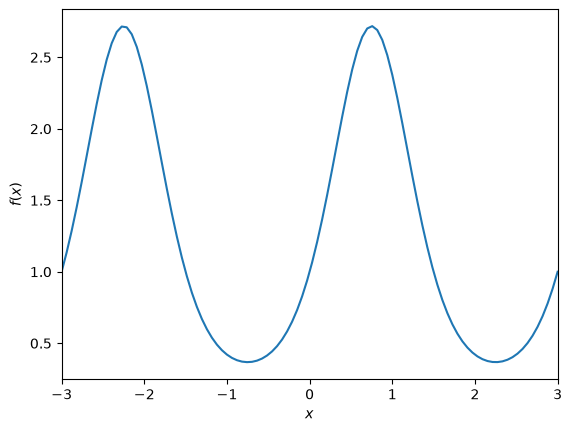
One of the core features of JAX is its support for automatic differentiation (AD; that’s what the “A” in JAX stands for). To differentiate a Python function using JAX, we start by writing the function using JAX’s numpy interface. In this case, let’s use a made up function that isn’t meant to be particularly meaningful:

\[ y = \exp\left[\sin\left(\frac{2\,\pi\,x}{3}\right)\right] \]

and then calculate the derivative using AD. For comparison, the symbolic derivative is:

\[ \frac{\mathrm{d}y}{\mathrm{d}x} = \frac{2\,\pi}{3}\,\exp\left[\sin\left(\frac{2\,\pi\,x}{3}\right)\right]\,\cos\left(\frac{2\,\pi\,x}{3}\right) \]

import jax
import jax.numpy as jnp

import numpy as np
import matplotlib.pyplot as plt


def func(x):
    arg = jnp.sin(2 * jnp.pi * x / 3)
    return jnp.exp(arg)


def symbolic_grad(x):
    arg = 2 * jnp.pi * x / 3
    return 2 * jnp.pi / 3 * jnp.exp(jnp.sin(arg)) * jnp.cos(arg)


x = jnp.linspace(-3, 3, 100)
plt.plot(x, func(x))
plt.xlabel(r"$x$")
plt.ylabel(r"$f(x)$")
plt.xlim(x.min(), x.max());

Then, we can differentiate this function using the jax.grad function. The interface provided by the jax.grad function may seem a little strange at first, but the key point is that it takes a function (like the one we defined above) as input, and it returns a new function that can evaluate the gradient of that input. For example:

grad_func = jax.grad(func)
print(grad_func(0.5))
np.testing.assert_allclose(grad_func(0.5), symbolic_grad(0.5))

2.4896522

One subtlety here is that we can only compute the gradient of a scalar function. In other words, the output of the function must just be a number, not an array. But, we can combine this jax.grad interface the jax.vmap function to evaluate the derivative of our entire function above:

plt.plot(x, jax.vmap(grad_func)(x), label="AD")
plt.plot(x, symbolic_grad(x), "--", label="symbolic")
plt.xlabel(r"$x$")
plt.ylabel(r"$\mathrm{d} f(x) / \mathrm{d} x$")
plt.xlim(x.min(), x.max())
plt.legend();

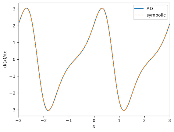
This example is pretty artificial, but I think that you can imagine how something like this would start to come in handy when your models get more complicated. In particular, I think that you’ll regularly find yourself experimenting with different choices of parameters, and it would be a real pain to be required to re-write all your derivative code for every new choice of parameterization.

Some more realistic examples

Straightforward AD with JAX works well as long as everything you’re doing can be easily and efficiently computed using jax.numpy. However, in many exoplanet and other astrophysics applications, we need to evaluate physical models that are frequently computed numerically, and things are less simple. A major driver of jaxoplanet is to provide some required custom operations to enable the use of JAX for exoplanet data analysis, including tasks like solving Kepler’s equation, or computing the light curve for a limb-darkened exoplanet transit. Most users shouldn’t expect to typically interface with these custom operations directly, but they are exposed through the jaxoplanet.core module.

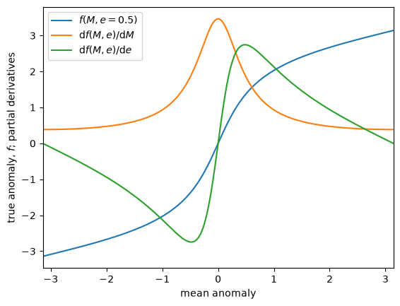
Solving Kepler’s equation

To start, let’s solve for the true anomaly for a Keplerian orbit, and its derivative using the jaxoplanet.core.kepler function:

from jaxoplanet.core import kepler

# The `kepler` function returns the sine and cosine of the true anomaly, so we
# need to take an `arctan` to get the value directly:
get_true_anomaly = lambda *args: jnp.arctan2(*kepler(*args))

# The following functions compute the partial derivatives of the true anomaly as
# a function of mean anomaly and eccentricity, respectively:
d_true_d_mean = jax.vmap(jax.grad(get_true_anomaly, argnums=0), in_axes=(0, None))
d_true_d_ecc = jax.vmap(jax.grad(get_true_anomaly, argnums=1), in_axes=(0, None))

mean_anomaly = jnp.linspace(-jnp.pi, jnp.pi, 1000)[:-1]
ecc = 0.5
true_anomaly = get_true_anomaly(mean_anomaly, ecc)
plt.plot(mean_anomaly, true_anomaly, label=f"$f(M,e={ecc:.1f})$")
plt.plot(
    mean_anomaly,
    d_true_d_mean(mean_anomaly, ecc),
    label=r"$\mathrm{d}f(M,e)/\mathrm{d}M$",
)
plt.plot(
    mean_anomaly,
    d_true_d_ecc(mean_anomaly, ecc),
    label=r"$\mathrm{d}f(M,e)/\mathrm{d}e$",
)
plt.legend()
plt.xlabel("mean anomaly")
plt.ylabel("true anomaly, $f$; partial derivatives")
plt.xlim(-jnp.pi, jnp.pi);

Of note, the Kepler solver provided by jaxoplanet does not use an iterative method like those commonly used for exoplanet fitting tasks. Instead, it uses a two-step solver which can be more efficiently parallelized using hardware acceleration like SIMD or a GPU. Even so, it is not computationally efficient or numerically stable to directly apply AD to this solver function. Instead, jaxoplanet uses the jax.custom_jvp interface to provide custom partial derivatives for this operation.

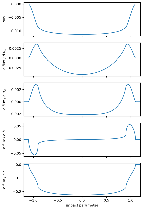
Limb-darkened transit light curves

jaxoplanet also provides a custom operation for evaluating the light curve of an exoplanet transiting a limb-darkened star, with arbitrary order polynomial limb darkening laws. This operation uses a re-implementation of the algorithms developed for the starry library in JAX. As above, we can use AD to evaluate the derivatives of this light curve model. For example, here’s a quadratically limb-darkened model and its partial derivatives:

from jaxoplanet.core.limb_dark import light_curve

lc = lambda u1, u2, b, r: light_curve(jnp.array([u1, u2]), b, r)
b = jnp.linspace(-1.2, 1.2, 1001)
r = 0.1
u1, u2 = 0.2, 0.3

_, axes = plt.subplots(5, 1, figsize=(6, 10), sharex=True)

axes[0].plot(b, lc(u1, u2, b, r))
axes[0].set_ylabel("flux")
axes[0].yaxis.set_label_coords(-0.15, 0.5)
for n, name in enumerate(["$u_1$", "$u_2$", "$b$", "$r$"]):
    axes[n + 1].plot(
        b,
        jax.vmap(jax.grad(lc, argnums=n), in_axes=(None, None, 0, None))(u1, u2, b, r),
    )
    axes[n + 1].set_ylabel(f"d flux / d {name}")
    axes[n + 1].yaxis.set_label_coords(-0.15, 0.5)
axes[-1].set_xlabel("impact parameter")
axes[-1].set_xlim(-1.2, 1.2);