Numerical precision

In general, we recommend setting JAX to double precision when working with jaxoplanet light curve functions

import jax

jax.config.update("jax_enable_x64", True)

Then, either to deal with very-precise datasets or for the sake of performance, users may want to adapt the precision of the light curve model. This can be done by changing the order parameter in most light_curve functions, which controls the number of points used for numerical integration.

Limb darkened light curve

To demonstrate that, let’s first compute a light curve at low order

from jaxoplanet.core.limb_dark import light_curve as light_curve

r = 1.0
b = 1.0
u = (1.0, 1.0)

calc = light_curve(u, b, r, order=10)

The simplest way to estimate the precision of this value is to compare it with one computed at large order

reference = light_curve(u, b, r, order=1500)

print(f"precision: {abs(calc - reference):.2e}")

precision: 1.08e-06

We can extend this approach further by computing the absolute error depending on the order of the numerical integration and the radius of the occultor

import jax.numpy as jnp


def estimate_precision(r=0.1):
    # values of b for which we expect the maximum error
    b = r if r > 1 else 1.0
    reference = light_curve(u, b, r, order=1500)

    def fun(order):
        calc = light_curve(u, b, r, order=order)
        result = jnp.abs(reference - calc)
        return max(result, 1e-16)

    return fun


orders = jnp.logspace(jnp.log10(5), jnp.log10(1000), 6).astype(int).tolist()

radii = [0.01, 0.1, 1.0]
with jax.disable_jit():
    precision = {r: [estimate_precision(r)(order) for order in orders] for r in radii}

And plot the results to identify an appropriate order for a given application

import matplotlib.pyplot as plt

for i, r in enumerate(radii):
    plt.plot(orders, precision[r], ".-", label=f"r={r}")

plt.yscale("log")
plt.xscale("log")
plt.xlabel("order of numerical integration")
plt.ylabel("absolute error")
plt.title("Limb darkening light curve precision")
_ = plt.legend()

Note

When setting the order parameter, keep in mind that the lower the order of the numerical integration, the faster the evaluation of the light curve function.

Starry light curve

The same thing can be done for starry light curves, but using the surface_light_curve function

from jaxoplanet.starry import Surface, Ylm
from jaxoplanet.starry.light_curves import surface_light_curve

# degree of the spherical harmonics map
l_max = 3

# a dummy surface described by unitary coefficients (not physical)
y = Ylm.from_dense(jnp.ones((l_max + 1) ** 2))
surface = Surface(y=y, u=(1.0, 1.0))

r = 1.0
b = 1.0

reference = surface_light_curve(surface=surface, y=b, r=r, z=1.0, order=1500)
calc = surface_light_curve(surface=surface, y=b, r=r, z=1.0, order=10)

print(f"precision: {abs(calc - reference):.2e}")

precision: 5.48e-05

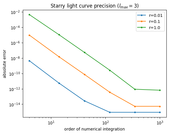
And as before

def estimate_precision(r=0.1):
    # values of b for which we expect the maximum error
    b = r if r > 1 else 1.0
    reference = surface_light_curve(surface=surface, y=b, r=r, z=1.0, order=1500)

    def fun(order):
        calc = surface_light_curve(surface=surface, y=b, r=r, z=1.0, order=order)
        result = jnp.abs(reference - calc)
        return max(result, 1e-16)

    return fun


with jax.disable_jit():
    precision = {r: [estimate_precision(r)(order) for order in orders] for r in radii}

for i, r in enumerate(radii):
    plt.plot(orders, precision[r], ".-", label=f"r={r}")

plt.yscale("log")
plt.xscale("log")
plt.xlabel("order of numerical integration")
plt.ylabel("absolute error")
plt.title(f"Starry light curve precision ($l_{{max}}={l_max}$)")
_ = plt.legend()