Transit Timing Variations

Similarly to exoplanet, jaxoplanet contains the ability to model transit timing variations for planetary systems. This tutorial follows from Fitting Transit Times from the exoplanet Python package.

Note

This tutorial requires some extra packages that are not included in the jaxoplanet dependencies.

Setup

We first setup the number of CPUs to use and enable the use of double-precision numbers with jax.

import jax
import numpyro

numpyro.set_host_device_count(2)
jax.config.update("jax_enable_x64", True)

Generating the data

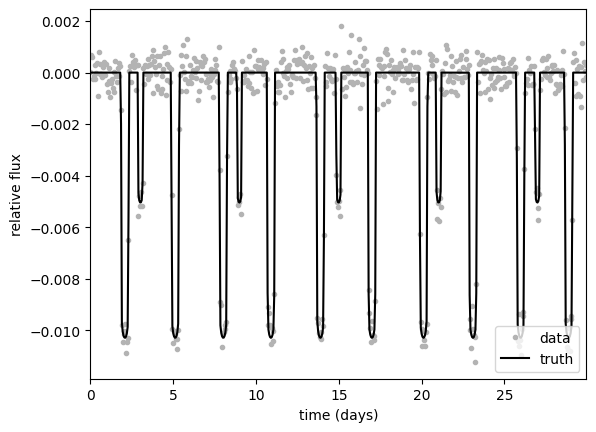
Let’s generate the light curve of a two-planet system featuring transit time variations.

TTVOrbit is an orbit object parameterized by the observables of a transiting system with transit time variations. On top of the TransitOrbit parameters, this orbit can be instantiated with a list of transit_times, omitting the need for a period and time of transit.

This is what our data model will look like

from jaxoplanet.orbits.ttv import TTVOrbit
from jaxoplanet.light_curves import limb_dark_light_curve


def orbit_and_lightcurve_model(time, params):
    transit_times = (params[f"transit_times_{i}"] for i in range(len(params["b"])))
    orbit = TTVOrbit(
        transit_times=transit_times,
        duration=params["duration"],
        impact_param=params["b"],
        radius_ratio=params["r"],
    )
    return orbit, limb_dark_light_curve(orbit, params["u"])(time)

Using the compute_expected_transit_times function, we can compute the expected transits of the system given the orbital parameters of the two planets.

import numpy as np
import jax.numpy as jnp
from jaxoplanet.orbits.ttv import compute_expected_transit_times

random = np.random.default_rng(11)

# true parmaters of the system
time = jnp.arange(0, 30, 0.05)  # day
true_periods = jnp.array([3, 6])  # day
true_t0s = jnp.array([2, 3])  # day

# computing expected transit times
expected_transit_times = compute_expected_transit_times(
    time.min(), time.max(), true_periods, true_t0s
)
n_planets = len(expected_transit_times)
planet_indices = jnp.arange(n_planets)
offset_factors = (3 / 24) - (planet_indices % 2) * 0.1
true_ttvs = []

for i, tt in enumerate(expected_transit_times):
    ttv = offset_factors[i] * jnp.sin(2 * jnp.pi * tt / 17)
    true_ttvs.append(ttv)

true_transit_times = tuple(
    tt + ttv for tt, ttv in zip(expected_transit_times, true_ttvs)
)

truth = {
    "transit_times_0": true_transit_times[0],
    "transit_times_1": true_transit_times[1],
    "b": jnp.array([0.5, 0.5]),
    "duration": jnp.array([0.5, 0.3]),
    "u": jnp.array([0.1, 0.06]),
    "r": jnp.array([0.1, 0.07]),
}

We can now generate and plot our data

import matplotlib.pyplot as plt

yerr = 5e-4
y_true_all = orbit_and_lightcurve_model(time, truth)[1]
y_true = jnp.sum(y_true_all, axis=-1)
y = jnp.array(y_true + yerr * random.normal(size=len(time)))

# Let's see what the light curve looks like
plt.plot(time, y, ".", c="0.7", label="data")
plt.plot(time, y_true, label="truth", c="k")
plt.xlabel("time (days)")
plt.ylabel("relative flux")
plt.xlim(time.min(), time.max())
_ = plt.legend(loc=4)

Model with NumPyro

We will now instantiate a NumPyro model in order to infer the properties of the system from the generated data.

Everything here is quite standard, but in the instance of a multi-planet system, we can supply a jax.numpy array of values for our priors, and we can apply the method to_event in order to tell Numpyro the dimensions are independent, that is, the period of planet 1 does not depend on the period of planet 2.

import numpyro_ext
import jax.numpy as jnp


def model(time, yerr, y=None):

    # For loop to account for each planet's transit times, with a Uniform prior
    # centered on the true transit times and lower/upper limits of 1 day.
    transit_times = []
    for i in range(2):
        transit_times.append(
            numpyro.sample(
                f"transit_times_{i}",
                numpyro.distributions.Uniform(
                    low=true_transit_times[i] - 1.0, high=true_transit_times[i] + 1.0
                ),
            )
        )

    # The duration
    logD = numpyro.sample(
        "logD",
        numpyro.distributions.Normal(jnp.log(truth["duration"]), 0.1).to_event(1),
    )
    duration = numpyro.deterministic("duration", jnp.exp(logD))

    # The radius ratio
    logR = numpyro.sample(
        "logR", numpyro.distributions.Normal(jnp.log(truth["r"]), 0.1).to_event(1)
    )
    r = numpyro.deterministic("r", jnp.exp(logR))

    # The impact parameter, note, for multi-planet systems, we need to pass in a
    # jax numpy array of values
    _b = numpyro.sample(
        "_b",
        numpyro.distributions.Uniform(
            low=jnp.array([0.0, 0.0]), high=jnp.array([1.0, 1.0])
        ).to_event(1),
    )
    b = numpyro.deterministic("b", _b * (1 + r))

    # The limb darkening coefficients
    u = numpyro.sample("u", numpyro_ext.distributions.QuadLDParams())

    params = {
        "b": b,
        "u": u,
        "r": r,
        "duration": duration,
        "transit_times_0": transit_times[0],
        "transit_times_1": transit_times[1],
    }

    orbit, y_pred_all = orbit_and_lightcurve_model(time, params)
    y_pred = jnp.sum(y_pred_all, axis=-1)

    # Here are some useful under the radar variables that we can access from TTVOrbit.
    # These are the linear ephemeris parameters and the TTVs.
    for i in range(2):
        numpyro.deterministic(f"t0_{i}", orbit.linear_t0[i])
        numpyro.deterministic(f"period_{i}", orbit.linear_period[i])
        numpyro.deterministic(f"ttvs_{i}", orbit.ttvs[i])

    # The likelihood function assuming Gaussian uncertainty
    numpyro.sample("obs", numpyro.distributions.Normal(y_pred, yerr), obs=y)

As in the the Fitting Transit Times tutorial, it might be a good idea to check the priors of your model.

Optimization

We will now optimize our model in preparation of sampling the posterior likelihood of the data

init_params = {
    **truth,
    "logD": jnp.log(truth["duration"]),
    "logR": jnp.log(truth["r"]),
    "_b": truth["b"] / (1 + truth["r"]),
}

run_optim = numpyro_ext.optim.optimize(
    model,
    init_strategy=numpyro.infer.init_to_value(values=init_params),
)

opt_params = run_optim(jax.random.PRNGKey(5), time, yerr, y=y)

Let’s plot the MAP model against the simulated data.

_, map_light_curve = orbit_and_lightcurve_model(time, opt_params)

plt.plot(time, y, ".", c="0.7", label="data")
plt.plot(time, y_true, "-k", label="truth")
plt.plot(time, map_light_curve.sum(1), "--", label="MAP model")
plt.xlabel("time [days]")
plt.ylabel("relative flux")
plt.legend(fontsize=10, loc=4)
plt.xlim(time.min(), time.max())
plt.tight_layout()

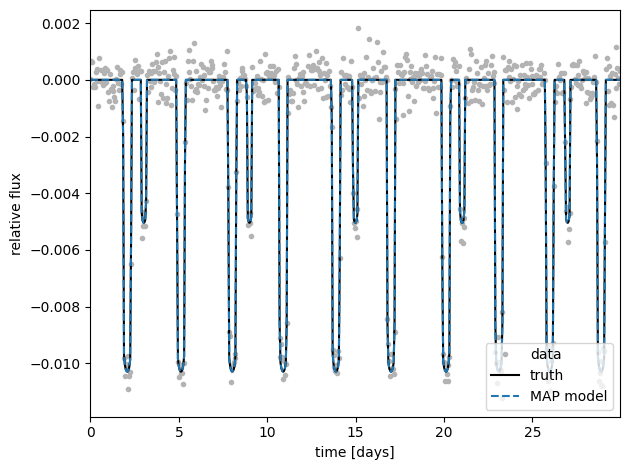
Looks good!

We are now going to have a quick look at the individual phase plots to demonstrate the issue with phasing planets exhibiting TTVs.

fig, ax = plt.subplots(2, 1, figsize=(7.5, 4))

map_t0s = [opt_params[f"t0_{i}"] for i in range(2)]
map_periods = [opt_params[f"period_{i}"] for i in range(2)]

for i, (period, t0) in enumerate(zip(map_periods, map_t0s)):
    folded_time = (time - t0 + 0.5 * period) % period - 0.5 * period
    ax[i].errorbar(
        folded_time,
        y - map_light_curve[:, 1 - i],
        yerr=yerr,
        fmt=".k",
        label="data",
        zorder=-1000,
    )
    ax[i].set_xlim(-0.5 * period, 0.5 * period)
    ax[i].set_xlabel("time since transit [days]")
    ax[i].set_ylabel("relative flux")
    ax[i].set_title("Planet 1")
    ax[i].legend()

That obviously doesn’t look great, but this is why we need to account for the TTVs, which TTVOrbit corrects under the hood.

Sampling

Let’s sample from the posterior.

sampler = numpyro.infer.MCMC(
    numpyro.infer.NUTS(
        model,
        dense_mass=True,
        regularize_mass_matrix=True,
        init_strategy=numpyro.infer.init_to_value(values=opt_params),
    ),
    num_warmup=500,
    num_samples=1000,
    num_chains=2,
    progress_bar=True,
)

sampler.run(jax.random.PRNGKey(1), time, yerr, y=y)

Let’s print the summary of our sampling, focusing on \(\hat{R}\) and the number of divergences encountered.

sampler.print_summary()

                        mean       std    median      5.0%     95.0%     n_eff     r_hat
             _b[0]      0.29      0.13      0.32      0.07      0.47    208.82      1.05
             _b[1]      0.23      0.15      0.21      0.01      0.45    396.46      1.00
           logD[0]     -0.71      0.01     -0.71     -0.72     -0.70    184.65      1.04
           logD[1]     -1.20      0.02     -1.19     -1.24     -1.17    161.22      1.01
           logR[0]     -2.31      0.01     -2.31     -2.32     -2.30    310.72      1.02
           logR[1]     -2.65      0.01     -2.65     -2.67     -2.64    640.09      1.01
transit_times_0[0]      2.09      0.00      2.09      2.08      2.09    210.21      1.03
transit_times_0[1]      5.12      0.00      5.12      5.12      5.12    960.59      1.00
transit_times_0[2]      8.02      0.00      8.02      8.02      8.03   1359.92      1.00
transit_times_0[3]     10.90      0.00     10.90     10.89     10.90    780.18      1.00
transit_times_0[4]     13.89      0.00     13.89     13.88     13.89    901.31      1.00
transit_times_0[5]     17.00      0.00     17.00     17.00     17.01   1015.93      1.00
transit_times_0[6]     20.11      0.00     20.11     20.11     20.12    413.00      1.03
transit_times_0[7]     23.10      0.00     23.10     23.09     23.10    804.17      1.01
transit_times_0[8]     25.98      0.00     25.98     25.97     25.98    777.25      1.00
transit_times_0[9]     28.88      0.00     28.88     28.88     28.89    136.23      1.02
transit_times_1[0]      3.02      0.00      3.02      3.01      3.03    551.64      1.00
transit_times_1[1]      9.00      0.00      9.00      8.99      9.00    139.04      1.01
transit_times_1[2]     14.98      0.01     14.98     14.97     14.99    332.04      1.00
transit_times_1[3]     21.03      0.00     21.03     21.02     21.03    409.64      1.00
transit_times_1[4]     26.99      0.00     26.99     26.99     27.00    335.92      1.01
              u[0]      0.08      0.06      0.07      0.00      0.16    594.64      1.00
              u[1]      0.11      0.11      0.10     -0.07      0.28    521.64      1.00

Number of divergences: 31

We can typically plot traces using the plot_trace function in the Arviz package

import arviz as az

inf_data = az.from_numpyro(sampler)

az.plot_trace(
    inf_data,
    var_names=["transit_times_0", "transit_times_1", "duration", "r", "b", "u"],
    backend_kwargs={"constrained_layout": True},
)
plt.show()

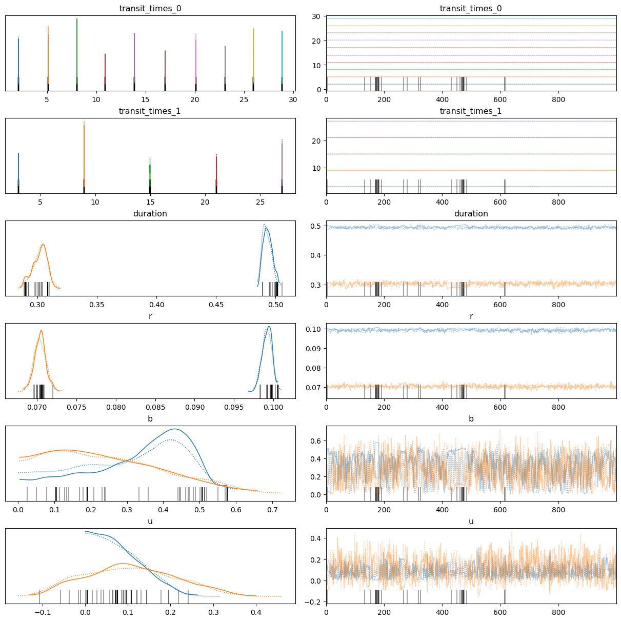
We have few divergences but not bad overall! Of course, for a real application these divergences must be investigated and the HMC should run on multiple and way longer chains.

TTV Plots

lets make some TTV plots to show we correctly identified the trend!

samples = sampler.get_samples()

fig, (ax1, ax2) = plt.subplots(2, 1, figsize=(10, 5), sharex=True)

q = np.percentile(samples["ttvs_0"], [16, 50, 84], axis=0)

ax1.fill_between(
    np.mean(samples["transit_times_0"], axis=0),
    q[0],
    q[2],
    color="C0",
    alpha=0.4,
    edgecolor="none",
)
ref = np.polyval(
    np.polyfit(true_transit_times[0], true_ttvs[0], 1), true_transit_times[0]
)
ax1.plot(true_transit_times[0], true_ttvs[0] - ref, ".k")
ax1.axhline(0, color="k", lw=0.5)
# ax1.set_ylim(np.max(np.abs(ax1.get_ylim())) * np.array([-1, 1]))

ax1.set_ylabel("$O-C$ [days]")

q = np.percentile(samples["ttvs_1"], [16, 50, 84], axis=0)
ax2.fill_between(
    np.mean(samples["transit_times_1"], axis=0),
    q[0],
    q[2],
    color="C1",
    alpha=0.4,
    edgecolor="none",
)
ref = np.polyval(
    np.polyfit(true_transit_times[1], true_ttvs[1], 1), true_transit_times[1]
)
ax2.plot(true_transit_times[1], true_ttvs[1] - ref, ".k", label="truth")
ax2.axhline(0, color="k", lw=0.5)
# ax2.set_ylim(np.max(np.abs(ax2.get_ylim())) * np.array([-1, 1]))

ax2.legend(fontsize=10)
ax2.set_ylabel("$O-C$ [days]")
ax2.set_xlabel("transit time [days]")
_ = ax1.set_title("posterior inference")

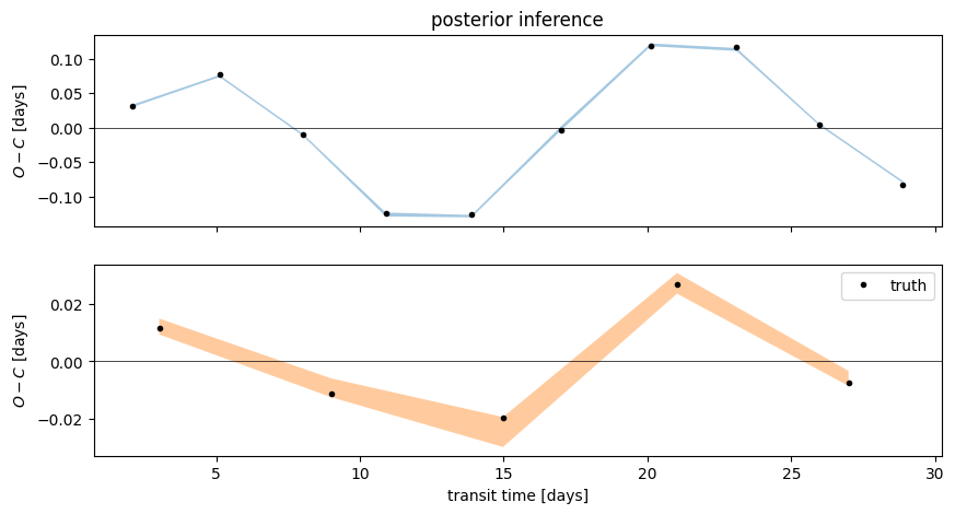
We can see the posterior is correctly predicting the true ttvs!