Quickstart

jaxoplanet is a Python package to model the unresolved light received from stellar and planetary systems. It implements most of the features from the exoplanet and starry packages built on top of JAX, allowing for hardware acceleration and interfacing with the tools from the JAX ecosystem.

Keplerian system

In jaxoplanet a Keplerian system can be instantiated with a Central object

from jaxoplanet.orbits.keplerian import System, Central

system = System(Central())  # a central object with some default parameters

and an orbiting Body added with

system = system.add_body(period=0.1)

Important

Note that period doesn’t have physical units here. Checkout the units convention to learn more about units in jaxoplanet.

system

System(
  central=Central(mass=1.0, radius=1.0, density=0.238732414637843),
  _body_stack=ObjectStack(...)
)

For the reminder of this notebook, let’s define a system consisting of an Earth-like planet orbiting a Sun-like star.

import astropy.units as u

sun = Central(
    radius=1.0,
    mass=1.0,
)

system = System(sun).add_body(
    semimajor=(1.0 * u.au).to(u.R_sun).value,
    radius=(1.0 * u.R_earth).to(u.R_sun).value,
    mass=(1.0 * u.M_earth).to(u.M_sun).value,
)

earth = system.bodies[0]

# checking the parameters of the system
system

System(
  central=Central(mass=1.0, radius=1.0, density=0.238732414637843),
  _body_stack=ObjectStack(...)
)

Note

Notice how physical quantities need to be converted to proper units before being passed to jaxoplanet functions. See the units convention for more details

Radial velocity

Then, one can access the relative position and velocity of the planet relative to the sun.

import jax.numpy as jnp
from matplotlib import pyplot as plt

# Get the position of the planet and velocity of the star as a function of time
t = jnp.linspace(0, 730, 5000)
x, y, z = earth.relative_position(t)
vx, vy, vz = earth.central_velocity(t)

Note

Axes and orbital parameters conventions follow that of the exoplanet package.

And plot the results

fig, axes = plt.subplots(2, 1, sharex=True)
ax = axes[0]
ax.plot(t, x, label="x")
ax.plot(t, y, label="y")
ax.plot(t, z, label="z")
ax.set_ylabel("earth position [$R_*$]")
ax.legend(fontsize=10, loc=1)

ax = axes[1]
ax.plot(t, vx, label="$v_x$")
ax.plot(t, vy, label="$v_y$")
ax.plot(t, vz, label="$v_z$")
ax.set_xlim(t.min(), t.max())
ax.set_xlabel("time [days]")
ax.set_ylabel("central velocity [$R_*$/day]")
_ = ax.legend(fontsize=10, loc=1)

Occultation light curve of limb darkened star

The light_curves.limb_dark.light_curve function can be used to compute the light curve of a limb darkened star with a polynomial profile, allowing to express linear, quadratic and more complex limb darkening laws.

Using the limb darkening coefficients of the Sun from Hestroffer and Magnan we compute the flux

from jaxoplanet.light_curves.limb_dark import light_curve

u_sun = (0.30505, 1.13123, -0.78604, 0.40560, 0.02297, -0.07880)
time = jnp.linspace(-0.5, 0.5, 1000)

flux = 1.0 + light_curve(system, u_sun)(time)

and plot the resulting light curve

plt.plot(time, flux)
plt.xlabel("time (days)")
_ = plt.ylabel("relative flux")

Non-uniform stars

jaxoplanet aims to match the features of starry, a framework to compute the light curves of systems made of non-uniform spherical bodies.

Warning

While being stable, computing starry light curves of non-uniform surfaces is still an experimental part of jaxoplanet.

Let’s define a Surface in the spherical harmonics basis (using the Ylm object) and visualize it

import numpy as np
from jaxoplanet.starry.ylm import Ylm
from jaxoplanet.starry.surface import Surface
from jaxoplanet.starry.visualization import show_surface

np.random.seed(42)
y = Ylm.from_dense([1.00, *np.random.normal(0.0, 2e-2, size=15)])

u_star = (0.1, 0.1)
surface = Surface(inc=1.0, obl=0.2, period=27.0, u=u_star, y=y)

plt.figure(figsize=(3, 3))
show_surface(surface)

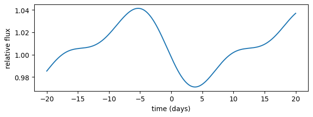
Rotational light curves

We can attach this surface to a body (like the Sun-like object we previously defined) and define a SurfaceSystem

from jaxoplanet.starry.orbit import SurfaceSystem

system = SurfaceSystem(sun, surface)

from which we compute the rotational light curve of the star

from jaxoplanet.starry.light_curves import light_curve

plt.figure(figsize=(6.5, 2.5))
time = jnp.linspace(-20, 20, 1000)
flux = light_curve(system)(time).T[0]

plt.plot(time, flux)
plt.xlabel("time (days)")
plt.ylabel("relative flux")
plt.tight_layout()

Occultation light curve

We can add a body to the system, having its own surface

system = SurfaceSystem(sun, surface)

secondary_surface = Surface(
    y=Ylm.from_dense([1.00, *np.random.normal(0.0, 1.0, size=15)])
)

system = system.add_body(
    semimajor=(40.0 * u.au).to(u.R_sun).value,
    radius=(20.0 * u.R_earth).to(u.R_sun).value,
    mass=(1.0 * u.M_earth).to(u.M_sun).value,
    impact_param=0.2,
    surface=secondary_surface,
)

and compute the occultation light curve of the system

t_start, t_end = -20, 20
n = 1000
time = jnp.linspace(t_start, t_end, n)
flux = light_curve(system)(time).T[0]

Let’s plot it and show the system over time

n_plots = 5
times = jnp.linspace(t_start, t_end, n_plots)
radius_ratio = system.bodies[0].radius / system.central.radius
gs = plt.GridSpec(2, n_plots)

plt.figure(figsize=(6.5, 4.0))

for i in range(n_plots):
    ax = plt.subplot(gs[0, i])
    phase = surface.rotational_phase(times[i])
    x, y = system.bodies[0].position(times[i])[0:2]
    show_surface(surface, ax=ax, theta=phase)
    circle = plt.Circle((x, y), radius_ratio, color="k", fill=True, zorder=10)
    ax.add_artist(circle)
    ax.set_xlim(-1.5, 1.5)

plt.subplot(gs[1, :])
plt.plot(time, flux)

plt.xlabel("time since transit (days)")
plt.ylabel("relative flux")
plt.tight_layout()